04 Apr Mass scaling for impact analysis
Mass scaling for Abaqus / Explicit
Abaqus/Explicit analyses have the tendency to require long simulation times in order to complete. Mass scaling can speed up the simulation without sacrificing simulation accuracy.
The explicit dynamics procedure is mainly used to solve two classes of problems: transient dynamic response calculations (like impact, crash and other simulations) and quasi-static simulations (like forming simulations). These kinds of simulations involve complex nonlinear effects (mainly complex contact conditions).
When used appropriately, mass scaling can often improve the computational efficiency while retaining the necessary degree of accuracy. However, the mass scaling techniques most appropriate for quasi-static simulations may be very different from those that should be used for dynamic analyses. In this post we will focus on a brief description of the mass scaling for impact analyses.
Mass scaling for dynamic events
Mass scaling for truly dynamic events should always occur only for a limited number of elements and should never significantly increase the overall mass properties of the model. One should check at the end of the simulation the percentage change in total model mass caused by mass scaling.
During an impact analysis the mass scaling option can be defined to only scale the masses of elements whose element stable time increments are less than a specified value.
Fixed versus variable mass scaling
Abaqus has different kind of mass scaling options, like fixed mass scaling (scaling the mass of few small elements at the beginning of the step) or variable mass scaling (scaling the mass of the critical elements during a step).
Mass scaling Finite Element example
The following example explains the effect of mass scaling with a simple example.
Mass scaling effect on simulation time
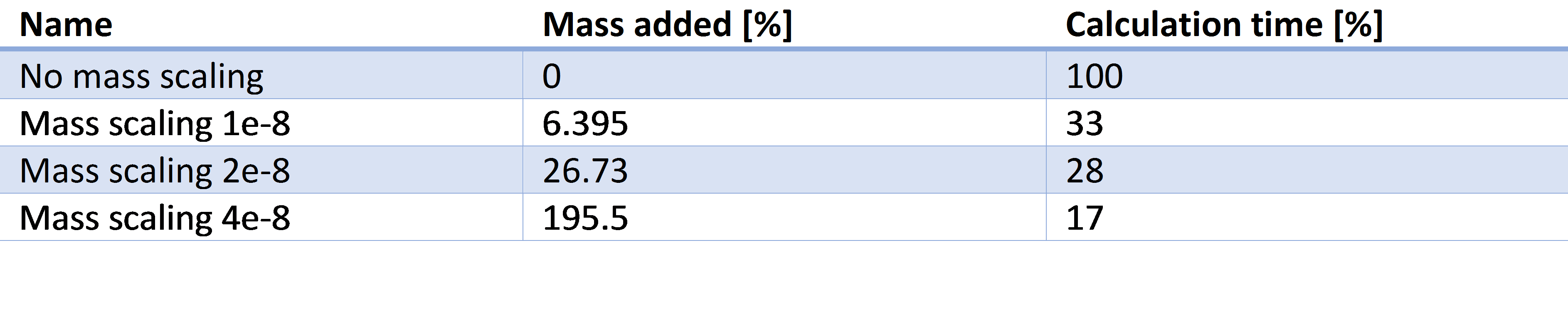
In the table, one can see 4 cases with different (or no mass scaling factor). When a mass scaling factor is applied, the mass of the elements with a time increment below a certain value are scaled. By adding a mass to these critical elements, the calculation time is decreased.
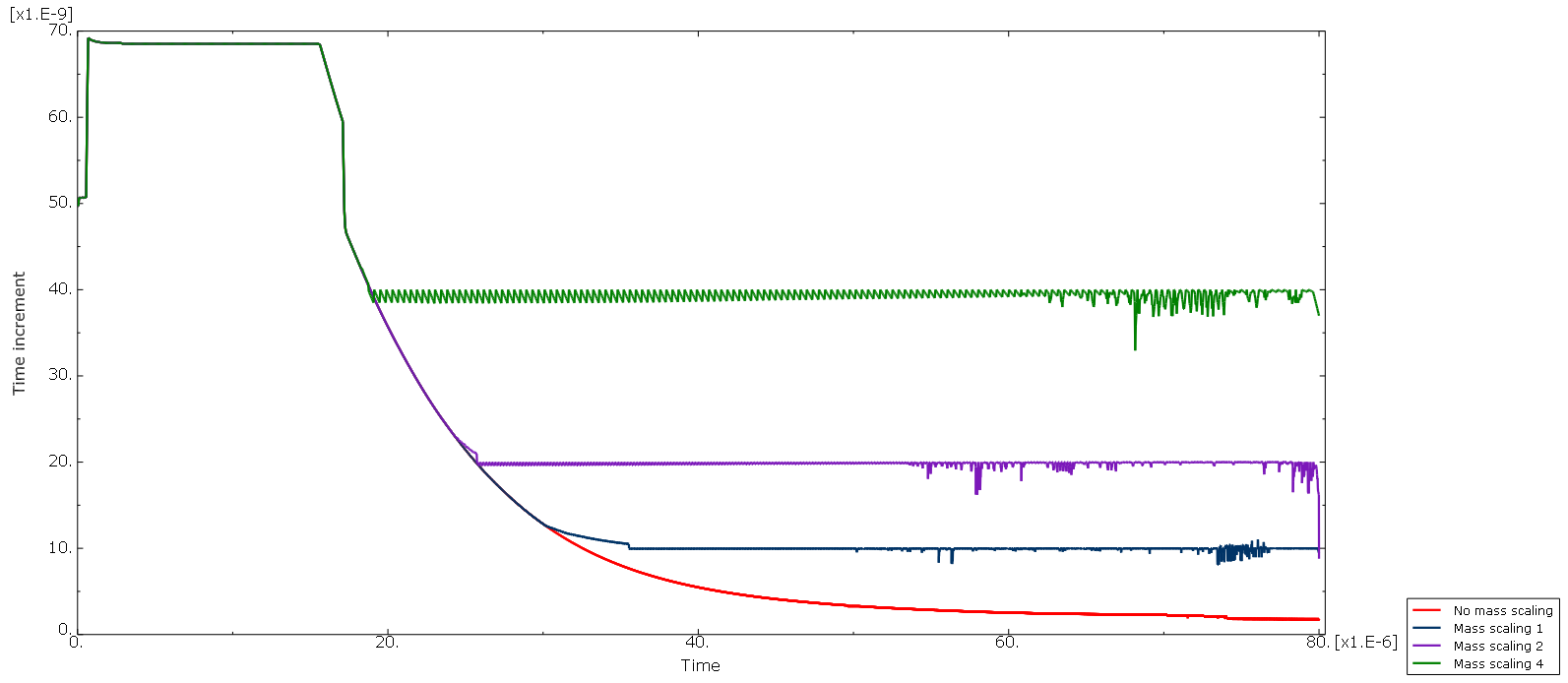
In the picture below, the time increment of the explicit analysis for the 4 different simulations is shown. The red curve shows the time increment when no mass scaling is applied. The blue, purple and green curve shows that the time increment remains constant when the critical value is reached.
Mass scaling energy balances
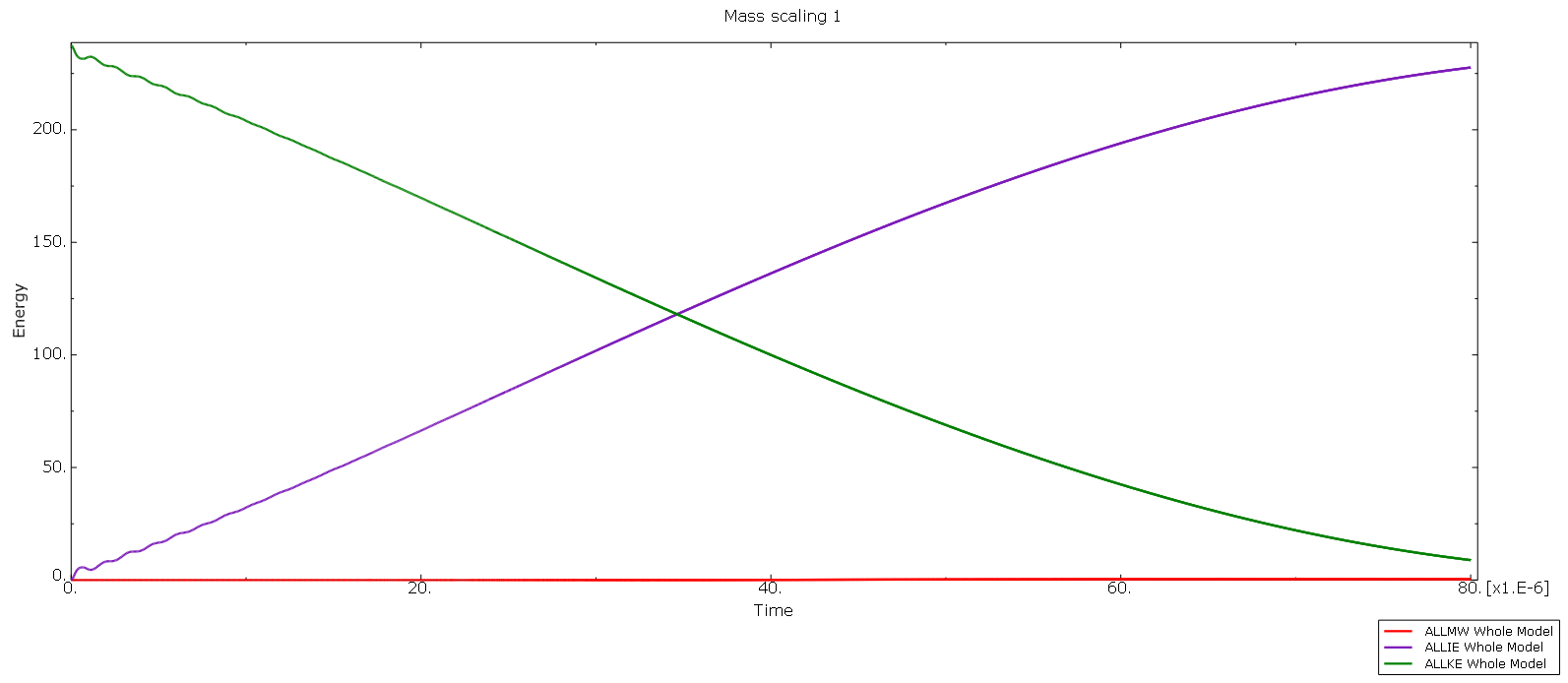
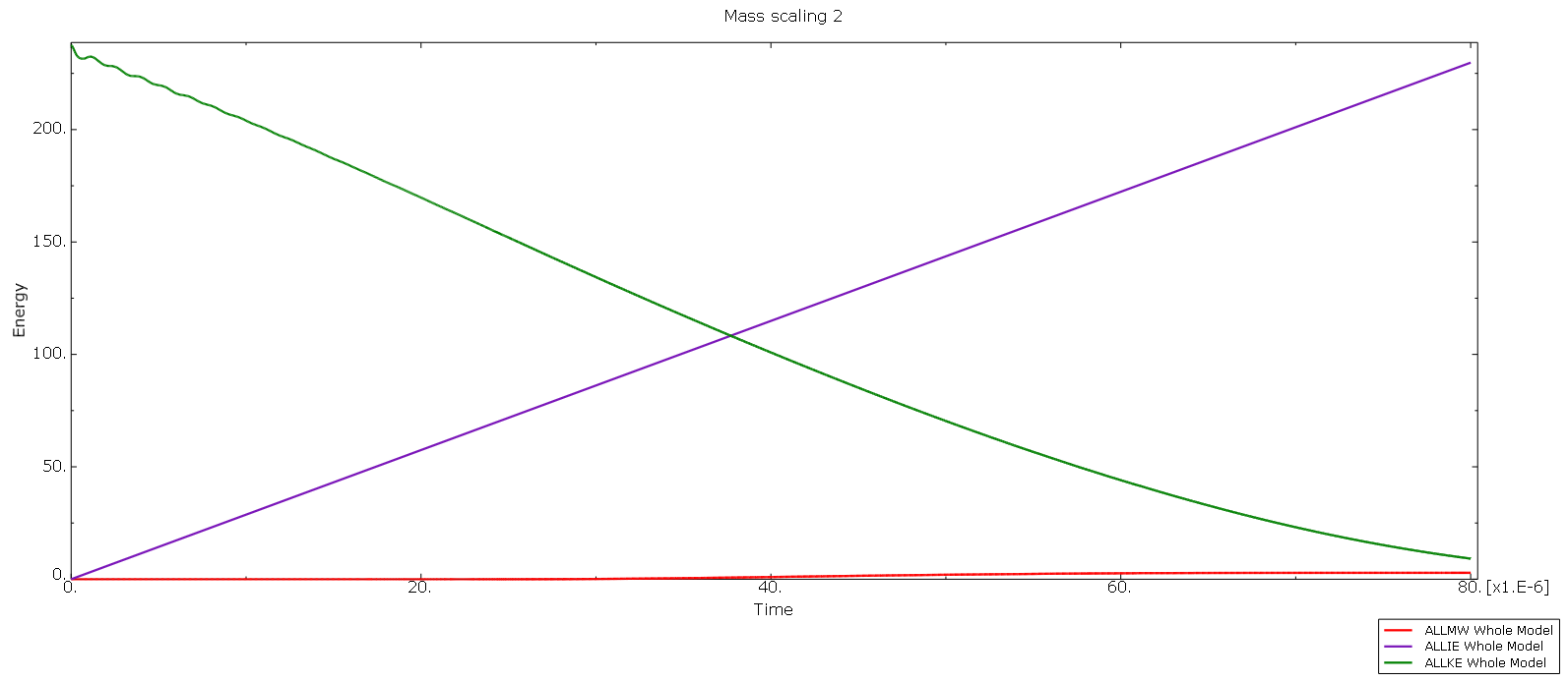
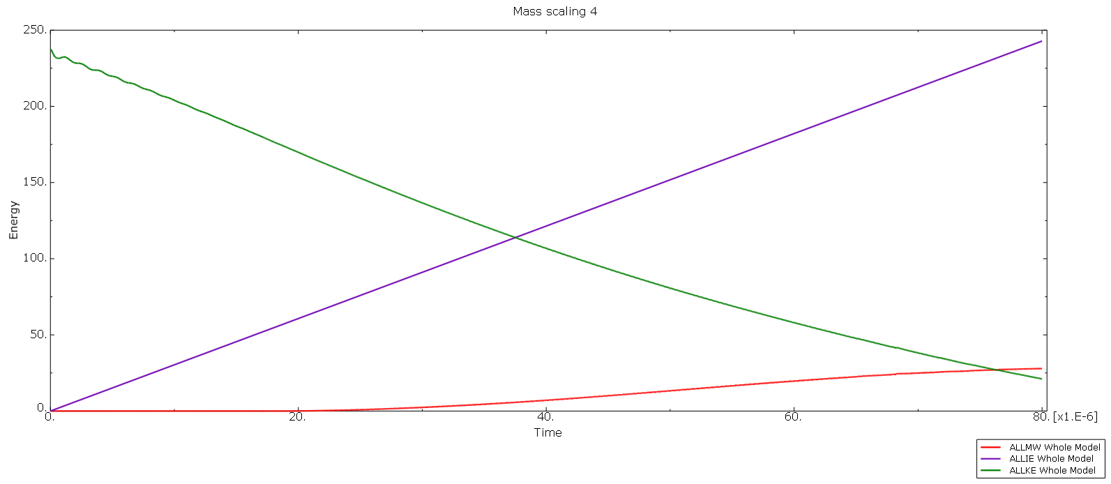
In the plots below you can see that the work done by propelling added mass (due to mass scaling) is having a more substantial influence on the energy balance (red curve – ALLMW). The green curve is the kinetic energy (ALLKE) and the purple curve is the internal energy (ALLIE).
Mass scaling influence on simulation results
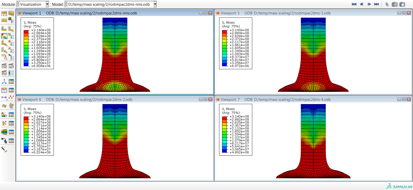
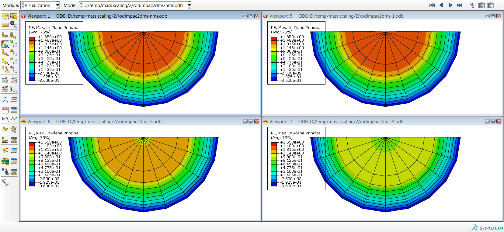
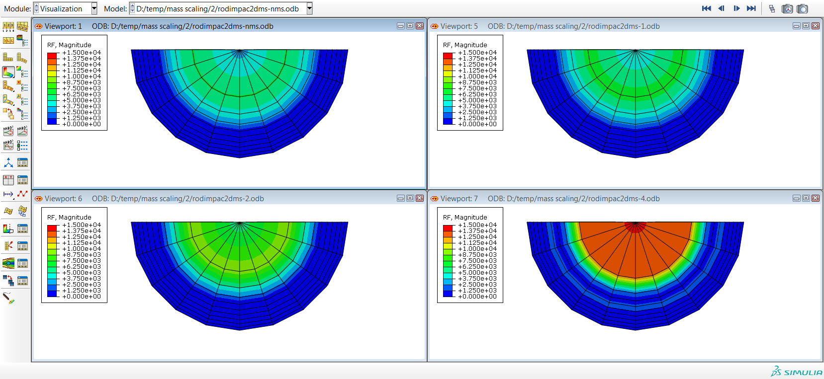
The stress, strain and reaction forces simulation results for the different mass scaling factors are shown below. The top left of each picture is the result with no mass scaling. The top right, bottom left and bottom right show the simulation results with a maximum time increment of 1e-8, 2e-8 and 4e-8, respectively. The influence of the mass scaling on the simulation accuracy is clearly visible. When the time increment cannot go below 1e-8, the results are still accurate, but for higher mass scaling values the simulations are becoming inaccurate.
Effect of mass scaling
The blog post describes the effect of mass scaling on impact simulations. Mass scaling can speed up impact simulations. But the user should investigate the % mass added due to mass scaling and energy balances to verify that its simulation results remain accurate.
If you have questions related to our post, feel free to contact us.

